Exploring line lengths in FluidDyn packages
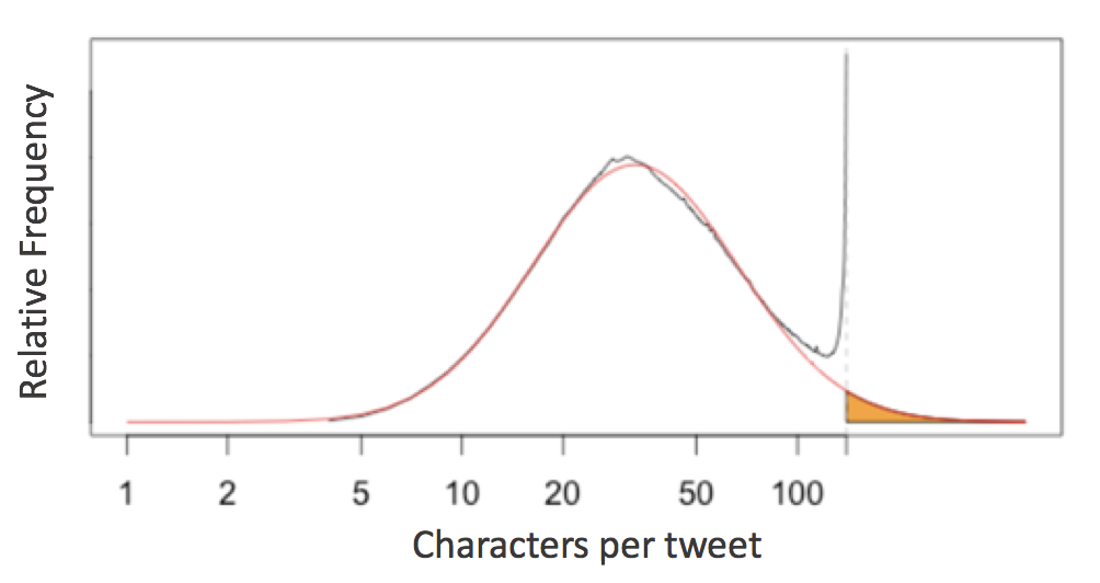
This analysis was inspired from Twitter’s interesting analysis of tweet lengths published on Twitter’s engineering blog. The gist of the analysis was this:
English language tweets display a roughly log-normal distribution of character counts, except near the 140-character limit - an evidence of cramming thoughts to fit 140 characters.
This prompts the question of the 79-character line limit suggested by Python’s PEP8 style guide:
Limit all lines to a maximum of 79 characters.
Jake VanderPlas invistigated this for scientific python packages. Let’s see how it affects FluidDyn packages!
Counting Lines in fluiddyn
To take a look at this, we first need a way to access all the raw lines of code in any Python package. In a standard system architecture, if you have installed a package you already have the Python source stored in your system.
import fluiddynWith this in mind, we can use the os.walk function to write a quick generator function that will iterate over all lines of Python code in a given package:
# Python 3.X
import os


def iter_lines(module):
    """Iterate over all lines of Python in module"""
    for root, dirs, files in os.walk(module.__path__[0]):
        for filename in files:
            if filename.endswith(".py"):
                with open(os.path.join(root, filename)) as f:
                    yield from f
This returns a generator expression that iterates over all lines in order; let’s see how many lines of Python code NumPy contains:
lines = iter_lines(fluiddyn)
len(list(lines))11340Given this we can find the lengths of all the lines and plot a histogram:
%matplotlib inline
import matplotlib.pyplot as plt
import numpy as np

plt.style.use("ggplot")
lengths = [len(line) for line in iter_lines(fluiddyn)]
plt.hist(lengths, bins=np.arange(max(lengths)), histtype="step", linewidth=1);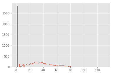
The distribution is dominated by lines of length 1 (i.e. containing only a newline character): let’s go ahead and remove these, and also narrow the x limits:
lengths = [len(line) for line in iter_lines(fluiddyn) if len(line) > 1]
plt.hist(lengths, bins=np.arange(125), histtype="step", linewidth=1);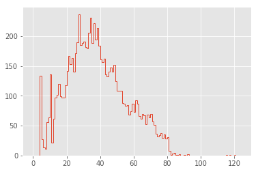
Now this is looking interesting!
Cleaning the Distribution
The first feature that pops out to me are the large spikes between 0 and 20 characters. To explore these, let’s look at the lines that make up the largest spike:
np.argmax(np.bincount(lengths))27We can use a list comprehension to extract all lines of length 13:
lines27 = [line for line in iter_lines(fluiddyn) if len(line) == 27]
len(lines27)237There are 237 lines in fluiddyn with a length of 27 characters. It’s interesting to explore how many of these short lines are identical.
The Pandas value_counts function is useful for this:
import pandas as pd

pd.value_counts(lines27).head(10)
if __name__ == '__main__':\n 48
from builtins import range\n 15
nb_cores_per_node = 16\n 3
sys.stdout.flush()\n 3
except ValueError:\n 3
print(*args, **kwargs)\n 2
for serie in self:\n 2
return self.shapeK\n 2
except AttributeError:\n 2
self.coef_norm = n\n 2
dtype: int64It’s clear that many of these duplicates are just a manifestation of if __name__ == '__main__': line and some imports from python-future package recurring at the beginning and the end of many modules.
lengths = [len(line) for line in set(iter_lines(fluiddyn))]
plt.hist(lengths, bins=np.arange(125), histtype="step", linewidth=1);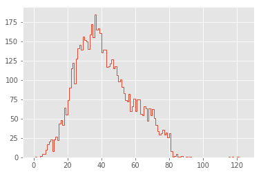
That’s a much cleaner distribution!
Comparison Between Packages
In order to aid comparison between packages, let’s quickly refactor the above histogram code into a function that we can re-use. In addition, we’ll add a vertical line at the PEP8’s maximum character count:
def hist_linelengths(module, ax):
    """Plot a histogram of lengths of unique lines in the given module"""
    lengths = [len(line.rstrip("\n")) for line in set(iter_lines(module))]
    h = ax.hist(lengths, bins=np.arange(125) + 0.5, histtype="step", linewidth=1.5)
    ax.axvline(x=79.5, linestyle=":", color="black")
    ax.set(
        title="{0} {1}".format(module.__name__, module.__version__),
        xlim=(1, 100),
        ylim=(0, None),
        xlabel="characters in line",
        ylabel="number of lines",
    )
    return h
Now we can use that function to compare the distributions for a number of well-known scientific Python packages:
%%capture --no-display
import fluiddyn, fluidsim, fluidfft, fluidimage, fluidlab, fluidcoriolis

modules = [fluiddyn, fluidsim, fluidfft, fluidimage, fluidlab, fluidcoriolis]

fig, ax = plt.subplots(2, 3, figsize=(14, 6), sharex=True)
fig.subplots_adjust(hspace=0.2, wspace=0.2)

for axi, module in zip(ax.flat, modules):
    hist_linelengths(module, ax=axi)

for axi in ax[0]:
    axi.set_xlabel("")
for axi in ax[:, 1:].flat:
    axi.set_ylabel("")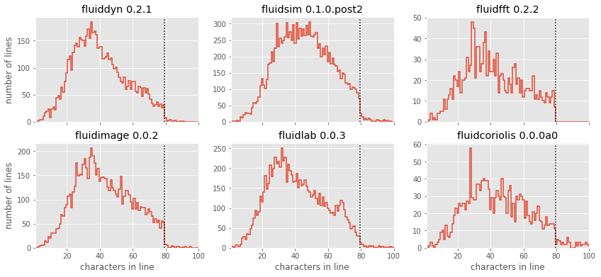
The results here are quite interesting: similar to Twitter’s tweet length analysis, we see that each of these packages have a somewhat smooth distribution of characters, with a “cutoff” at or near the 79-character PEP8 limit! There is a reasonable adherence to PEP8 standards, but unlike the results from Jake’s analysis of other scientific pacakges, there are no recognizable “bumps” near the 79-character limit. fluidfft has the most cleanest tail with absolutely 0 lines with above 79 characters - a luxury of being the newest package.
But one package stands out: fluidsim displays some noticeable spikes at a few intermediate line lengths; let’s take a look at these:
lines = set(iter_lines(fluidsim))
counts = np.bincount([len(line) for line in lines])
np.argmax(counts)50The large spike reflects the approximately 300 lines with exactly 50 characters; printing some of these and examining them is interesting:
[line for line in lines if len(line) == 50][:10]["def load_bench(path_dir, solver, hostname='any'):\n",
' subcommand = compute_name_command(module)\n',
" it = group_state_phys.attrs['it']\n",
' freq_complex = np.empty_like(state_spect)\n',
' shape_variable=(33, 18),\n',
' sim.oper.KX[ikx, iky],\n',
" z_fft = self.state_spect.get_var('z_fft')\n",
' Fy_reu = -urx * px_etauy - ury * py_etauy\n',
'=================================================\n',
' PZ2_fft = (abs(Frot_fft)**2)*deltat/2\n']Maybe not so interesting after all, just a coincidence! :)
Modeling the Line Length Distribution
Following the Twitter character analysis, let’s see if we can fit a log-normal distribution to the number of lines with each character count. As a reminder, the log-normal can be parametrized like this:
Here is the number of counts, is the median of the peak of the distribution, and controls the distribution’s width.
We can implement this using the lognorm distribution available in scipy:
from scipy import stats


def lognorm_model(x, amplitude, mu, sigma):
    return amplitude * stats.lognorm.pdf(x, scale=np.exp(mu), s=sigma)


x = np.linspace(0, 100, 1000)
plt.plot(x, lognorm_model(x, 1000, 3.5, 0.7));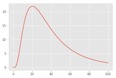
That seems like an appropriate shape for the left portion of our datasets; let’s try optimizing the parameters to fit the counts of lines up to length 50:
from scipy import optimize

counts, bins, _ = hist_linelengths(fluiddyn, ax=plt.axes())
lengths = 0.5 * (bins[:-1] + bins[1:])


def minfunc(theta, lengths, counts):
    return np.sum((counts - lognorm_model(lengths, *theta)) ** 2)


opt = optimize.minimize(
    minfunc, x0=[10000, 4, 1], args=(lengths[:50], counts[:50]), method="Nelder-Mead"
)
print("optimal parameters:", opt.x)

plt.fill_between(lengths, lognorm_model(lengths, *opt.x), alpha=0.3, color="gray");
optimal parameters: [6.53825230e+03 3.68332005e+00 4.59205976e-01]
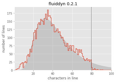
Seems like a reasonable fit! From this, you could argue (as the Twitter engineering team did) that the line lengths might “naturally” follow a log-normal distribution, if it weren’t for the artificial imposition of the PEP8 maximum line length.
For convenience, let’s create a function that will plot this lognormal fit for any given module:
def lognorm_model(x, theta):
    amp, mu, sigma = theta
    return amp * stats.lognorm.pdf(x, scale=np.exp(mu), s=sigma)


def minfunc(theta, lengths, freqs):
    return np.sum((freqs - lognorm_model(lengths, theta)) ** 2)


def lognorm_mode(amp, mu, sigma):
    return np.exp(mu - sigma**2)


def lognorm_std(amp, mu, sigma):
    var = (np.exp(sigma**2) - 1) * np.exp(2 * mu + sigma**2)
    return np.sqrt(var)
def hist_linelengths_with_fit(module, ax, indices=slice(50)):
counts, bins, _ = hist_linelengths(module, ax)
lengths = 0.5 * (bins[:-1] + bins[1:])
opt = optimize.minimize(
minfunc,
x0=[1e5, 4, 0.5],
args=(lengths[indices], counts[indices]),
method="Nelder-Mead",
)
model_counts = lognorm_model(lengths, opt.x)
ax.fill_between(lengths, model_counts, alpha=0.3, color="gray")
# Add text describing mu and sigma
A, mu, sigma = opt.x
mode = np.exp(mu - sigma**2)
ax.text(
0.22,
0.15,
"mode = {0:.1f}".format(lognorm_mode(*opt.x)),
transform=ax.transAxes,
size=14,
)
ax.text(
0.22,
0.05,
"stdev = {0:.1f}".format(lognorm_std(*opt.x)),
transform=ax.transAxes,
size=14,
)
return opt.xNow we can compare the models for each package:
modules = [fluiddyn, fluidsim, fluidfft, fluidimage, fluidlab, fluidcoriolis]

fig, ax = plt.subplots(2, 3, figsize=(14, 6), sharex=True)
fig.subplots_adjust(hspace=0.2, wspace=0.2)

fits = {}

for axi, module in zip(ax.flat, modules):
    fits[module.__name__] = hist_linelengths_with_fit(module, ax=axi)


for axi in ax[0]:
    axi.set_xlabel("")
for axi in ax[:, 1:].flat:
    axi.set_ylabel("")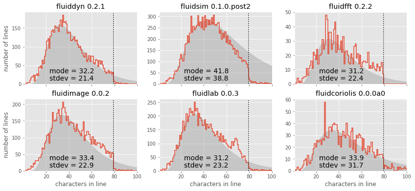
It is also interesting to use these summary statistics as a way of describing the “essence” of each package, in order to compare them directly:
ha = {"fluidfft": "right", "fluidlab": "right", "pandas": "right"}
va = {"fluidfft": "top"}
for name, fit in sorted(fits.items()):
    mode = lognorm_mode(*fit)
    std = lognorm_std(*fit)
    plt.plot(mode, std, "ok")
    plt.text(
        mode,
        std,
        " " + name + " ",
        size=14,
        ha=ha.get(name, "left"),
        va=va.get(name, "bottom"),
    )
plt.xlabel("mode of model", size=14)
plt.ylabel("std. deviation of model", size=14)
plt.xlim(27, 45)
plt.ylim(21, 41);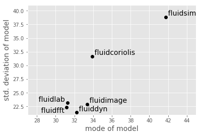
This notebook originally appeared as a post on the blog Pythonic Perambulations. The code content is MIT licensed.
This modified post was written entirely in the Jupyter notebook. You can download this notebook, or see a static view on nbviewer.